Experimenting with nVIDIA Rapids (1)

Unleashing the potential of Nvidia Rapids: Accelerating the ML Algorithms with cuML library

Intro to Rapids

nVIDIA Rapids is an open-source suite of GPU-accelerated Python software libraries that provide high-performance data science and machine learning tools. It gives faster performance at scale across data pipelines. There are generally 4 major ways to get started with nVIDIA Rapids which include:

cuML ~ for Machine Learning
cuGraph ~ for Graph Analytics
Spark (RAPIDS) ~ a RAPIDS Accelerator for Apache Spark
cuDF ~ for Data Analytics

In our first blog, I'll be majorly focusing on the usage of cuML library in order to accelerate the training and performance of Machine Learning algorithms like Linear Regression, RandomForestRegressor, etc. This will also include a little bit of use of cuDF as well. We'll take a well-focused & deeper look into what cuDF basically is in one of my upcoming blogs, alone let this blog be about cuML and how it overpowers CPU-based Scikit Learn using its GPU-accelerated suite.

To keep you all on track with our code, I'll be demonstrating the process and running the code on Google Colaboratory.

In Google Colab, you can perform an "Environment Sanity Check" to assess the status of the GPU you've been allocated and a lot more by running the following command.

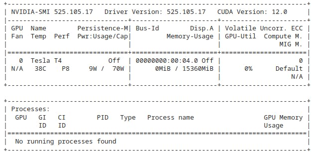
!nvidia-smi

(smi ~ System Management Interface)

The !nvidia-smi command is used to check the status and information about NVIDIA GPUs (Graphics Processing Units) in a Linux environment, including Google Colab. It provides details about the currently installed NVIDIA GPU(s), such as the GPU model, driver version, GPU utilization, temperature, and memory usage.

You must be given a Tesla T4, P4, or P100. Your output must look similar to this.

To make sure that you go along with the latest stable update of RAPIDS, I recommend you to work on the rapids-conda-colab-template regularly managed & updated by the organization itself.

Go to RAPIDS and click on Docs. Go on Installation Guide and look for the sub-heading Cloud Instance GPUs where you'll find a link stating Google CoLab w/ Conda. Click on that link and you'll be redirected to an .ipynb notebook in Google CoLab consisting of the latest stable update of Rapids and there, after successfully installing Rapids on CondaCoLab, you may start with the training of your desired machine learning algorithm.

Importing the required libraries

import cudf
from cuml import make_regression, train_test_split
from cuml.linear_model import LinearRegression as cuLinearRegression
from cuml.metrics.regression import r2_score
from sklearn.linear_model import LinearRegression as skLinearRegression

PS: I have also included the sklearn(scikit-learn) library in order to show you all the differnce between the performance of CPU and GPU since sklearn is a CPU-based library.

Generating Random Regression Data

Now, it is time to generate the data:

In order to generate some random regression data, we need a number of samples, number of features and random state:

n_samples = 2**10
n_features = 399

random_state = 23

%%time
X, y = make_regression(n_samples=n_samples, n_features=n_features, random_state=random_state)

X = cudf.DataFrame(X)
y = cudf.DataFrame(y)[0]

X_cudf, X_cudf_test, y_cudf, y_cudf_test = train_test_split(X, y, test_size = 0.2, random_state=random_state)

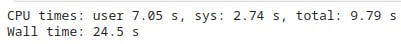
PS: %%time command is a built-in magic command used to measure the execution time of a specific code cell. When you prepend a cell with %%time, it will run the code in the cell and display information about how long it took to execute. This will generate an output similar to this:

Now, let us copy the dataset from GPU memory to host(CPU) memory. Well, this is being done as we'll be comparing the CPU & GPU later on in this demonstration.

X_train = X_cudf.to_pandas()
X_test = X_cudf_test.to_pandas()
y_train = y_cudf.to_pandas()
y_test = y_cudf_test.to_pandas()

Fit, Predict & Evaluate The Scikit-Learn Model

To fit:

%%time
ols_sk = skLinearRegression(fit_intercept=True,
                            # normalize=True,
                            n_jobs=-1)

ols_sk.fit(X_train, y_train)

PS: normalize attribute has been deprecated for the skLinearregression function. But still works in the cuML library.

To predict:

%%time
predict_sk = ols_sk.predict(X_test)

For the r2 score metrics:

%%time
r2_score_sk = r2_score(y_cudf_test, predict_sk)

Fit, Predict & Evaluate The cuML Model

To fit:

%%time
ols_cuml = cuLinearRegression(fit_intercept=True,
                              normalize=True,
                              algorithm='eig')

ols_cuml.fit(X_cudf, y_cudf)

To predict:

%%time
predict_cuml = ols_cuml.predict(X_cudf_test)

For r2 score metrics:

%%time
r2_score_cuml = r2_score(y_cudf_test, predict_cuml)

Time To Compare The Results

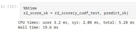
Since I have used the %%time command in every code block, you may be able to see the time it took to execute that respective block of code. You must a noticeable difference between the time it took to fit, predict and to check the r2 score metrics for scikit-learn and cuML libraries. Look below for an instance:

This shows the system time as 2.08ms for scikit-learn model.

And this shows the system time as 23 micro-seconds for cuML model.

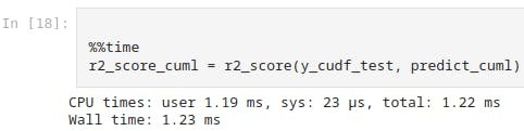
This further clarifies how cuML accelerates the Machine Learning Algorithms as it operates on the basis of GPU which offers high efficiency, scalability and faster performance when dealing with amounts of data counting 100 or 1k times more than what we have just assumed in this demonstration.

You may take a hands-on approach by your own-selves. Just click on this Epsit's Github link and open the Google CoLab through my uploaded file. You'll also find some handwritten notes for your reference. Also feel free to contribute there or raise any issue if you want to.

So hey fellow sailors, let's see where our sail takes us next...

My Experiments With Code